Spam Detection Using Machine Learning
Development Enviroment
For the Spam detection project, I decided to use Google Colab, which runs virtually and is accessible from any browser. It only requires a login with a google account to run the Notebook
Libraries
The following libraries has been used:
- pandas
- sklearn
- numpy
- nltk
- re
- seaborn
- matplotlib.pyplot
Colab Notebook
The Colab Nootbook can be downloaded here: Spam Detection.
Dataset Exploration
For Spam Detection, I used a Kaggle Dataset containing an extensive list of emails. First, I reviewed the dataset, printed out the dimension and an overview of how it looks and found out that the distribution of the emails needed to meet the requirements for my classification. It needed to include more spam emails. So I had to do a resampling of the dataset to achieve an equal class distribution, which means I got the same amount of spam and ham emails.
Preprocessing
Before implementing any classification algorithm, the emails had to be prepared in the right format through a process called preprocessing. During this process, a number of steps were taken to clean the text of irrelevant information. Firstly, stop words, which are common words that do not carry much meaning, were removed. Numbers, symbols, and anything that was not a letter were also removed. The next step was to apply lemmatization, which involved reducing each word to its base form.
Once the text had been cleaned, it was converted into a matrix of numbers, which allowed for feature scaling using the MinMaxScaler technique. Additionally, the chi-square test was used for selecting meaningful features and reducing the dimension of the dataset. This involved calculating the chi-square statistic for each feature and selecting only the features with the highest scores. By doing so, the most relevant features were retained, while eliminating irrelevant features that could have a negative impact on the performance of the classification algorithm.
Classification
After the preprocessing step, the text data was transformed into numerical features using the scikit-learn library. The following classification algorithms were then implemented:
- Naive Bayes: This is a widely used classifier for text classification. The naive Bayes classifier is easy to implement and computationally efficient. It performs well on relatively small datasets compared to other algorithms. It is based on Bayes’ theorem, which assumes that all the features are independent of each other.
- Decision Trees: This algorithm works by breaking down the data through a series of questions, creating a complex decision boundary. However, care must be taken to avoid overfitting. The deeper the decision tree, the more complex the decision boundary becomes.
- K-Nearest Neighbors: KNN is a lazy learner that memorizes the training data and uses the closest points to a new data point to classify it. It is a simple algorithm but can be computationally expensive for large datasets.
- Support Vector Machine (SVM): This is a popular algorithm for classification tasks. It finds the best decision boundary by maximizing the margin between the classes. The data points closest to the decision boundary are called support vectors, and they are used to define the decision boundary. SVMs are powerful and can handle both linear and nonlinear data.
- Random Forest: This is an ensemble learning algorithm that builds a collection of decision trees. Each tree is trained on a random subset of the training data and a random subset of the features. The final prediction is made by combining the predictions of all the trees in the forest. Random forests help to reduce overfitting and improve the generalization performance of the model.
- Gradient Boosting: This is another powerful machine learning algorithm that is used for regression, classification, and other predictive modeling tasks. It is an ensemble method that combines multiple weak learners to create a strong learner. In Gradient Boosting, each weak learner is trained on the residual error of the previous learner. The final prediction is made by summing the predictions of all the weak learners. Gradient Boosting is a popular choice for large datasets and can handle both linear and nonlinear data.
Training using K-Nearest Neighbors and Gradient Boosting takes long time running on the Colab Notebook.
Performance
To evaluate the performance of the classification algorithms, I used various metrics such as precision, recall, f1-score, confusion matrix, PR-curve, and ROC-curve.
- Precision: This metric measures the proportion of correctly classified positive instances out of all instances that the model predicted as positive. A higher precision indicates that the classifier is less likely to classify non-spam emails as spam.
- Recall: This metric measures the proportion of actual positive instances that were correctly classified by the model. A higher recall indicates that the classifier is less likely to classify spam emails as non-spam.
- F1-score: This metric is a combination of precision and recall and provides a single score that reflects both metrics. It is the harmonic mean of precision and recall and is a useful metric to evaluate the performance of a classification model.
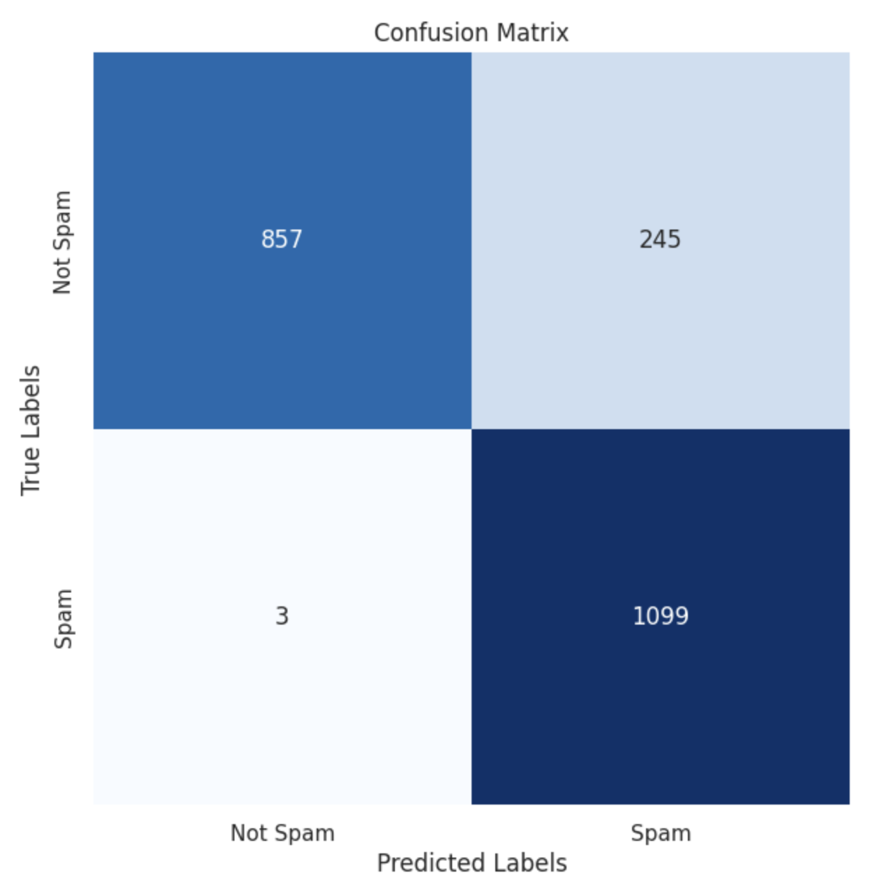
- Confusion Matrix: It is a table used to evaluate the performance of a classification model. A confusion matrix consists of four entries: true positives (TP), true negatives (TN), false positives (FP), and false negatives (FN). The entries in the matrix can be used to compute various metrics such as precision and recall.
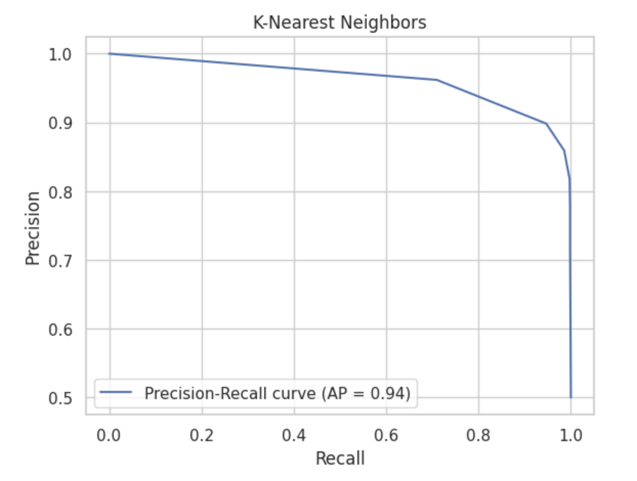
- PR-Curve: This curve shows the trade-off between precision and recall for different classification thresholds. It is a useful metric when dealing with imbalanced datasets where the number of negative examples is much higher than the number of positive examples.
- ROC-Curve: This curve shows the trade-off between true positive rate (TPR) and false positive rate (FPR) for different classification thresholds. It is a useful metric when the cost of false positives and false negatives is similar, and the dataset is balanced.
| Predicte Positive | Predicte Negative | |
|---|---|---|
| Actual Positive | True Positive (TP) | False Negative (FN) |
| Actual Negative | False Positive (FP) | True Negative (TN) |
The entries in the diagonal (TP and TN) represent correct predictions, while the off-diagonal entries (FP and FN) represent incorrect predictions.
- Precision Recall Curve: It plots the precision and recall scores of a model for different classification thresholds.
Results
This is the graphical overview of the classifications performnance:
Naive Bayes


Decision Tree


K-Nearest Neighbors


Support Vector Machines


Random Forest


Gradient Boosting


